


After following packets through QEMU and the Arista leaves, I wanted to watch the network without opening a console on every device. I wanted to select CE1 in Grafana, find GigabitEthernet2, and see whether its traffic, errors or discards changed while Longhorn moved data between sites.
Getting a collector pod to start would not answer that question. Its requests had to reach the devices’ management routing tables, the devices had to permit them, and storage had to accept the measurements. Then the dashboard had to show an interface I could recognize from the router’s command-line interface (CLI).
I finished with fresh measurements from all 28 routers and switches and a network dashboard whose interface names match the CLI. I also added the cluster and storage measurements I needed beside those graphs, then organized Grafana around the systems I would investigate. I extended that collection to BGP peers, IS-IS neighbors and Cisco BFD sessions, checking the results against the CLI before trusting the dashboard. This post follows the path into Grafana, including the gaps I found in the devices’ SNMP tables and the event history I still need for brief routing failures.
Part 6 covers the original K3s installation and Nautobot-backed Ansible inventory. The free companion, The Interfaces Were Up. The Packets Had Stopped., explains the QEMU and Arista packet failures I repaired first. Here I build on those foundations to collect and display the network measurements.
K3s is the Kubernetes distribution running the applications. Longhorn stores their persistent volumes, VictoriaMetrics stores measurements over time, and Grafana displays them. Argo CD keeps the Kubernetes resources aligned with their declarations in Git. SNMP supplies the device measurements; OpenTelemetry (OTel) carries them to storage.
A place to run the monitoring system
The cluster has three masters in DC-A and six workers across DC-B and DC-C. The masters run the Kubernetes API and embedded etcd, the database holding cluster state. They remain together because the packet fixes did not establish consistently low latency under cross-site storage load. Loss of DC-A still means loss of the control plane.
The hosts use K3s v1.30.5+k3s1 and bond0 for Flannel traffic. I disabled the bundled Traefik and ServiceLB so the ingress components described later have their own Git-managed configuration. Flannel connects the pod networks over VXLAN. Its MTU is 8950 over the 9000-byte host data interfaces.
I needed each correction to survive the next deployment. Host configuration, device commands and Kubernetes resources have different owners, so I kept their sources separate:
Repository sourceWhat it controlsblog-sandbox/ansible/Ubuntu networking, K3s and standalone BINDblog-sandbox/golden-config/templates/Device configuration generated from Nautobotblog-sandbox/telemetry/Generated SNMP collector values and dashboardblog-sandbox-argo-cd/bootstrap/argocd-values.yamlArgo CD’s own Helm installationblog-sandbox-argo-cd/apps/Child Applications discovered by the rootblog-sandbox-argo-cd/values/Workload Helm configurationblog-sandbox-argo-cd/observability/Cluster and storage collection, health alerts and dashboard folders
The Ansible workflow obtains host addresses and roles from Nautobot. Neither a second static inventory nor manual edits to generated device configurations are needed.
Giving the recovered cluster a declared application state
Part 6 had already modeled host and K3s configuration in Git. For Kubernetes applications, I needed a controller to keep reconciling those declarations after the initial install. With GitOps, I put the desired resources in a repository and let the controller work toward that state. Reverting a commit can restore earlier resource declarations; it does not restore application data from a volume.
Argo CD represents each managed application with an Application custom resource: a repository, a path or chart, a revision, and a destination. Point one Application at a directory of other Application manifests and it becomes an app-of-apps. I apply the root once, then add workloads through files in Git.
Standing up Argo CD
Helm packages Kubernetes resource definitions into a chart, with a values file supplying configuration. I use the chart mirror prepared in Part 6 and keep Argo CD’s settings in bootstrap/argocd-values.yaml. The examples below assume both repositories are checked out on the automation host and kubectl is using the lab’s Kubernetes context.
I placed Argo CD’s components in DC-A, on the same three nodes that already hold etcd and the API server. The node selector below limits placement to that site. The toleration permits these pods to run on nodes reserved for the control plane:
global:
  nodeSelector:
    kubernetes.io/os: linux
    topology.kubernetes.io/zone: dc-a
  tolerations:
    - key: node-role.kubernetes.io/control-plane
      operator: Equal
      value: "true"
      effect: NoSchedule
DC-A was reserved for the control plane in Part 6. Argo CD is a deliberate exception. The application controller talks continuously to the API, and keeping its repo-server and Redis in the same site avoids spreading that internal traffic across DC-A, DC-B and DC-C. I checked the available capacity before placing it there. The storage and application workloads run on the workers in DC-B and DC-C. The host-level monitoring collectors described later run on the nodes they monitor, including the masters.
The bootstrap values also select docker.io/library/redis, which uses the Docker Hub cache configured in Part 6. With the values in place, install Argo CD from the pinned chart:
cd /home/ubuntu/blog-sandbox-argo-cd
helm upgrade --install argocd \
  http://192.168.3.21:8888/helm/argo-cd-10.8.0.tgz \
  --namespace argocd --create-namespace \
  --values bootstrap/argocd-values.yaml \
  --wait --timeout 10m
kubectl -n argocd get pods
The chart version and mirror address belong to this lab. If you’re adapting the repository, check those values and the DC-A node labels against your cluster first. Before continuing, confirm the Argo CD pods are Ready.
Making the first sync wait for storage
Argo CD keeps comparing Git declarations with live Kubernetes resources. One root Application, applied by hand once, watches a directory in blog-sandbox-argo-cd and auto-discovers everything else:
spec:
  source:
    repoURL: https://github.com/byrn-baker/blog-sandbox-argo-cd.git
    targetRevision: main
    path: apps
    directory:
      recurse: false
  syncPolicy:
    automated:
      prune: true
      selfHeal: true
The first two children were Longhorn at sync-wave 1 and VictoriaMetrics/Grafana at wave 2. The monitoring deployment adds cluster-observability at wave 3, snmp-metrics at wave 4 and otel-snmp at wave 5. MetalLB and the ingress resources follow at waves 9 through 12. A sync wave is a numbered group applied before a higher-numbered group. Storage must be ready before the applications request volumes, and the stores should be ready before the collector starts exporting.
Argo CD needs Application health handling for the parent to use child health in this pattern. I installed the customization from bootstrap/argocd-values.yaml and checked it in the live argocd-cm.
The chart-based child Applications point repoURL at the mirror directory containing index.yaml. The chart and targetRevision fields select the package. For Longhorn, those fields are:
repoURL: http://192.168.3.21:8888/helm/
chart: longhorn
targetRevision: 1.12.1
A direct .tgz URL works in the Helm install command above, but it isn’t a Helm repository URL for an Argo Application.
Longhorn also needs this setting in values/longhorn-values.yaml:
preUpgradeChecker:
  jobEnabled: false
This disables an upgrade-check hook that otherwise runs before its service account exists during the initial Argo installation. The Longhorn issue explains the hook conflict.
Once Argo is Ready, apply the root and watch its children:
kubectl apply -f bootstrap/root-app.yaml
kubectl -n argocd get applications -w
Synced means the deployed resources match Git; Healthy means they meet Argo’s health checks. Confirm Longhorn and VictoriaMetrics have both statuses before moving on to collection. The collector also needs the credential Secret created in the generation step below. The Application health customization controls the initial ordering through the root. It doesn’t serialize every later update: existing children can auto-sync independently.
Argo’s own bootstrap values sit outside the root’s apps/ path. To change those settings later, rerun the Helm command with the updated values.
A running application still needed working storage
Longhorn keeps volume replicas, copies on separate workers, and attaches the volume to the application pod. A PersistentVolumeClaim (PVC) is the application’s request for storage. Kubernetes attachment state and Longhorn replica health answer different questions, so I checked both:
# From the automation host with its existing lab Kubernetes context
kubectl get nodes -o wide
kubectl get pvc -A
kubectl get volumeattachments
kubectl -n longhorn-system get volumes.longhorn.io
kubectl -n longhorn-system get pods
Before starting collection, check that the claims are Bound, the volumes are attached where needed, and Longhorn reports healthy replicas. Also check free space in both the Ubuntu guests and the hypervisor’s storage pool. Space inside a VM doesn’t tell you whether the underlying pool can accept more writes.
Grafana’s values use a Recreate deployment strategy, which stops the old pod before starting its replacement, and a longer startup allowance for database initialization. Those settings live in values/victoria-metrics-values.yaml. They let Kubernetes wait for Grafana to initialize its persistent database before treating a slow start as a failure.
Getting the devices to answer
SNMP, the Simple Network Management Protocol, lets a collector request measurements such as interface byte counters, errors and uptime. My network scope was 13 Cisco IOS-XE routers and 15 Arista EOS switches. Nautobot also held ten Ubuntu servers, but those were outside this device-polling rollout.
I already used Nautobot to generate device configuration, so I used the same model for SNMP access. A config context supplies structured values that templates turn into commands. The community, contact and allowed source network were shared across all seven network-device roles; location came from each device’s own record. One context was enough. The community below is a placeholder:
snmp:
  ro_community: "<snmp-read-only-community>"
  contact: "byrn-baker demo-lab"
  acl_source: "192.168.3.0/24"
  acl_source_wildcard: "0.0.0.255"
I used SNMPv2c for this lab’s first collection path, with read-only access and a source access control list (ACL), which permits requests from specified addresses. A community is the shared string the collector presents to an SNMPv2c agent. It travels without encrypted authentication. The ACL limits where requests may originate; it does not give v2c the security properties of SNMPv3. The choice kept this first deployment’s scope small, and it should remain an explicit lab tradeoff.
I permit the management VLAN because the collector can move between workers. On the captured polling path, requests left the worker’s eth0 interface using its management IP. When adapting the ACL, check the source address of actual SNMP requests; a pod’s internal address may be translated before the device sees it.
The ACL syntax differs between platforms:
{% raw %}
{# ios/snmp.j2 #}
ip access-list standard ACL-SNMP-RO
 permit {{ config_context.snmp.acl_source.split('/')[0] }} {{ config_context.snmp.acl_source_wildcard }}
{% endraw %}
{% raw %}
{# eos/snmp.j2 #}
ip access-list standard ACL-SNMP-RO
   10 permit {{ config_context.snmp.acl_source }}
{% endraw %}
The two templates look similar, but the devices expect different address syntax. EOS accepts CIDR, which writes a network and prefix length together, such as 192.168.3.0/24. IOS expects the network address followed by a wildcard mask, which marks the address bits the rule can ignore.
I validate the rendered commands before deploying them:
# From the blog-sandbox checkout
make ci
make ci-full
The first command checks template structure. The second adds Batfish configuration checks, which can catch invalid device syntax even when Jinja renders successfully. The active compliance definitions live in jobs/gc_compliance_setup/__init__.py.
EOS needed the management VRF and the ACL
A Virtual Routing and Forwarding instance (VRF) has its own routing table. The EOS management interfaces belong to MGMT-VRF, so SNMP also has to be enabled in that routing context to answer requests there. The template correction emits one snmp-server vrf <name> line per unique VRF on a modeled Management interface. The resulting device configuration includes:
ip access-list standard ACL-SNMP-RO
   10 permit 192.168.3.0/24
snmp-server community <snmp-read-only-community> ro ACL-SNMP-RO
snmp-server vrf MGMT-VRF
I deploy both the snmp and acl features. The SNMP feature covers snmp-server commands, but the access list is a separate configuration block. Deploying just the community’s ACL reference doesn’t install the restriction itself.
After syncing the source into Nautobot, I regenerate intended configuration, collect fresh backups, run compliance and generate Config Plans. I check one device per platform before expanding to the fleet, with Fail Job on Task Failure enabled. Live reads and successful polls confirmed the VRF binding and ACL on all 15 EOS devices.
Check that the settings will survive a restart
Running configuration is active now; startup configuration is what the device loads after reboot. I compare both, because polling can work even when the saved configuration is incomplete:
show running-config
show startup-config
Check the SNMP community, ACL and EOS management VRF in both outputs. If a save is needed, review the rest of the running configuration first so unrelated changes aren’t saved accidentally:
copy running-config startup-config
Then reconnect and read startup configuration again. Nautobot’s intended files, backups and per-device job logs help with that comparison, but a successful job status doesn’t replace the device readback.
Generate the collector from the same device model
The generator selects IOS-XE and EOS devices from Nautobot, using their roles, management addresses, sites and SNMP contexts. The ten Ubuntu servers are excluded from this 28-device scope. I use one collector with two export destinations, so writing to two stores does not double the polling load on devices. The completed configuration has 28 device receivers and three additional BGP-only receivers for the SERVERS VRF, covered later in the post.
The following commands are the repository’s generation workflow. Start in the parent directory of adjacent blog-sandbox and blog-sandbox-argo-cd checkouts. They require its Python dependencies, the existing Nautobot credentials in the environment, a Kubernetes context pointing at the lab, and the observability namespace and VictoriaMetrics operator already installed. --sync-secret writes the externally managed Kubernetes credential Secret; this is a deployment step, not a read-only preview.
cd blog-sandbox
python3 telemetry/generate_snmp.py \
  --canary CE1 DCA-Leaf01 \
  --output ../blog-sandbox-argo-cd/values/otel-snmp-values.yaml \
  --sync-secret
pytest telemetry/test_generate_snmp.py -q
The canary selects one Cisco router and one Arista leaf from the same model. After checking their measurements, the full-fleet generation uses the same command without --canary CE1 DCA-Leaf01. I review the generated non-secret diff, render it with the pinned chart and validate the collector configuration with the pinned binary before publishing the values to the Argo repository. The root Application discovers the declared children; I do not apply a separate collector Deployment by hand.
The generator runbook records dependencies, pinned artifacts and credential rotation. Credentials go into network-snmp-credentials in namespace observability, while Git holds the references. Synchronizing that Secret does not change the SNMP community on a router or switch.
The collector uses memory-backed export queues. A restart can lose queued samples and creates a polling gap; this deployment does not promise lossless delivery during outages. Freshness, polling errors and queue metrics make those gaps visible.
Following a measurement into storage
Once the canaries answered, I could follow their measurements through the rest of the path. The OpenTelemetry Collector polls every 60 seconds, with staggered starts so all devices do not answer at once. It forwards samples using OTLP, the OpenTelemetry Protocol, over HTTP to two VictoriaMetrics stores. The existing store holds cluster metrics; the second keeps a separate, longer history for SNMP. Grafana queries the stored measurements.
13 IOS-XE routers + 15 EOS switches
                 |
        SNMP over management VLAN
                 |
           OTel Collector
                 |
             OTLP/HTTP
            /         \
  cluster metrics     SNMP history
            \         /
               Grafana
The fleet rollout produced samples from all 28 devices in both stores. Each device had at least five uptime samples in the five-minute check, and the oldest latest sample was less than 60 seconds old. The collector’s export queues were empty, its refused-point counters were zero, and it reported no failed exports. That established more than a running pod: device replies had become stored measurements I could query.
The dedicated SNMP store is configured for 547 days of retention on a 20 GiB volume. I kept it separate because extending retention for every Kubernetes metric would have a different storage cost. The cluster store retains its existing one-month setting. A retention setting does not prove that the disk can hold that much history; I still need to measure growth. A time series is one metric with a particular set of labels, such as incoming bytes on one interface of one device. More series and more samples consume more space.
The interface name had to mean the same thing on the router
The first dashboard returned measurements, but its legends exposed the entire label set: device, address, interface index, abbreviated name and collector metadata. That was information the storage system needed, presented as though it were an interface name. I still had to work out which line belonged to the port I wanted to inspect.
I compared the collected names with show interfaces on all 28 devices. SNMP’s interface Management Information Base, or IF-MIB, gives each interface row an index and several descriptive fields. A MIB defines the objects a device exposes through SNMP. The index identifies a row for polling and joining counters; it is not a useful label for a graph.
The two name fields also differed. On CE1, ifName contained Gi2, while ifDescr contained GigabitEthernet2. On DCA-Leaf01, both contained Ethernet1. My collector already stored ifDescr in the interface label, so I could correct the presentation without changing the stored measurements.

I made the Device and Interface selectors use those full names. Traffic legends now pair the device with its interface, and the status table has three useful columns: Device, Interface and Interface status. Numeric states render as Up, Down or the corresponding named condition. Error and discard panels show rates in errors/s and discards/s. The internal labels remain available for diagnosis without taking over the dashboard.
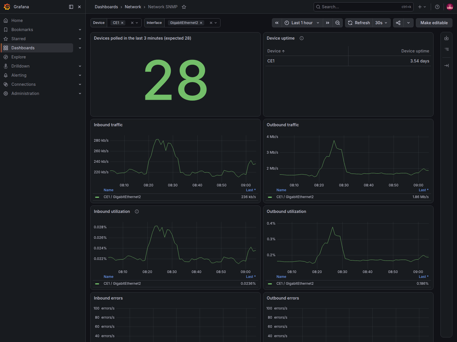
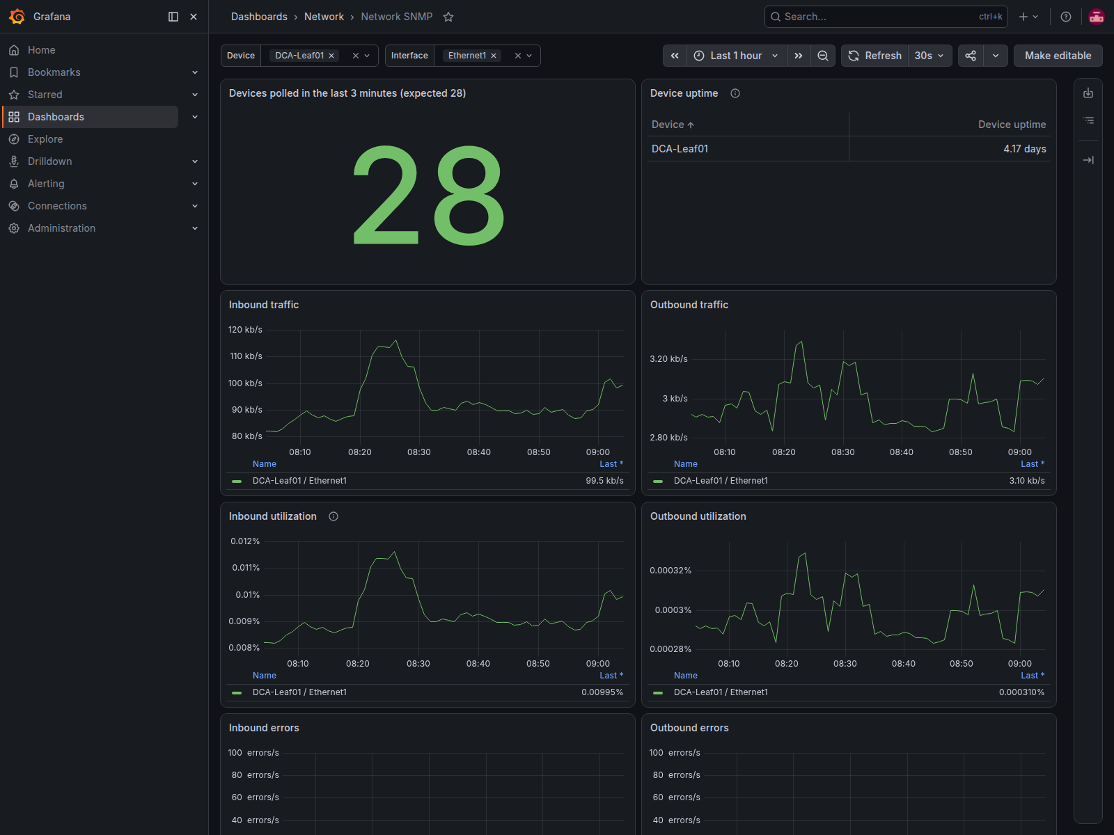
Here I selected CE1 and GigabitEthernet2. The traffic panels follow that selection; the freshness counter still checks all 28 devices. The Arista view uses the same layout with DCA-Leaf01 / Ethernet1.
Why 372 SNMP rows became 318 displayed interfaces
The name comparison exposed another distinction: an SNMP interface row does not always represent another port. The stored data contained 372 rows. Of those, 28 described the Multiprotocol Label Switching (MPLS) layer on Cisco interfaces, and 26 were IOS Null0 or VoIP-Null0 sinks, internal destinations for discarded traffic. The remaining 318 names appeared in the devices’ show interfaces output.
MPLS forwards traffic using labels attached to packets. Its SNMP rows describe that protocol layer, so they could represent traffic already counted on the underlying interface. Plotting them as additional links would make the network appear busier than it was. They also lacked error and discard counters. On the inspected SP1 row, a direct request returned noSuchInstance: the requested object identifier, or OID, did not have a value there. The physical interface returned a real counter. Missing and zero meant different things.
I excluded the MPLS rows and IOS null sinks from the normal interface selectors and panels. I kept the raw measurements and a separate table identifying MPLS rows without error counters. That left a view I could compare with the CLI without throwing away diagnostic data.
There was one gap in the other direction. Each Arista leaf showed an internal Vlan4097 in its CLI output, but those nine interfaces were absent from the collected IF-MIB rows. I documented the exception rather than adding empty graphs that would imply collection was working for them.
Keeping dashboard changes in Git
I made these changes in telemetry/network_dashboard.py, the dashboard’s source. The generated JSON travels inside a ConfigMap in the Collector’s Helm values, then reaches Grafana through Argo CD. Editing the dashboard only in Grafana would leave the next deployment able to replace my changes.
The generator escapes Grafana’s legend placeholders so Helm preserves them when rendering the ConfigMap. I check the rendered chart as well as the dashboard JSON, because the dashboard passes through both formats before Grafana reads it.
For this presentation change, I used the generator’s dashboard-only mode from the blog-sandbox checkout:
python3 telemetry/generate_snmp.py --dashboard-only \
  --output ../blog-sandbox-argo-cd/values/otel-snmp-values.yaml
This updates the dashboard while preserving the receiver configuration and credential revision. Review and publish the values through the Argo repository, then check the result in Grafana with one Cisco interface and one Arista interface selected. Both should show full names, readable status values and explicit rate units.
My browser and query checks covered both platforms. The audit and screenshots record the CLI comparison and rendered result.
Giving each part of the lab a place in Grafana
Once I could recognize the network interfaces, I needed to make the rest of Grafana useful too. The chart had placed its dashboards together in General. Looking for a storage problem meant searching past cluster views, dashboards for the metrics stores and panels for operating systems I wasn’t running.
I organized them around where I would go to investigate a problem:
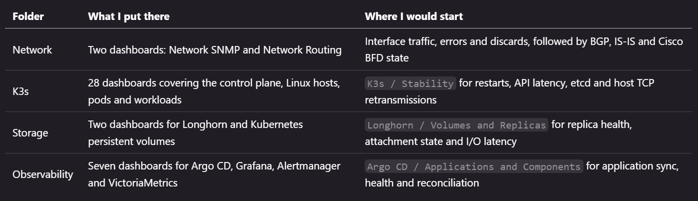
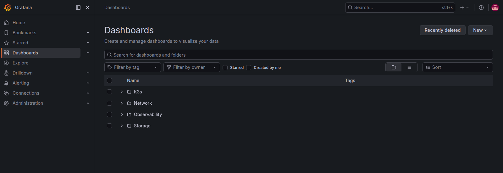
That left 39 dashboards and none in General. I removed the Windows, AIX, macOS, multi-cluster and Prometheus-server dashboards because those systems weren’t deployed here. The existing Linux and Kubernetes detail views stayed available when I needed to move beyond the overview.
A folder needed data behind it
The control-plane dashboards exposed a collection gap. K3s runs etcd, the scheduler and controller manager inside its server process. The scheduler chooses where pods run; the controller manager keeps resources aligned with their requested state. The chart’s normal discovery expected separate component pods, so those scrapes had no targets. A scrape is the collector’s request to a component’s metrics endpoint. An empty target list meant I had no measurement, not that the component had stopped.
I added a small vmagent collector on each master to read the existing loopback listeners: port 2381 for etcd, 10257 for the controller manager and 10259 for the scheduler. Loopback is the host’s local network connection. These collectors share the host’s network namespace so they can reach it without exposing the listeners elsewhere or restarting K3s. They send samples to the existing cluster metrics store every 30 seconds. The configuration is in observability/control-plane.yaml.
Longhorn’s endpoint was available too, but its NetworkPolicy, the Kubernetes rule controlling incoming connections, blocked the monitoring agent. I added a rule admitting that agent to the managers’ shared API and metrics port, then collected all six managers. I also added metrics from five Argo CD components, including its application controller and repository server. The collection manifests keep the endpoint selection and access rules together.
Now I can start with a container restart in the K3s folder and compare its time window with API latency and etcd disk writes. The Storage folder shows whether a volume was rebuilding or experiencing slow I/O. Network gives me the interface counters for the same window. That comparison helps narrow the next check; a host-wide retransmission counter still cannot identify which connection lost data.
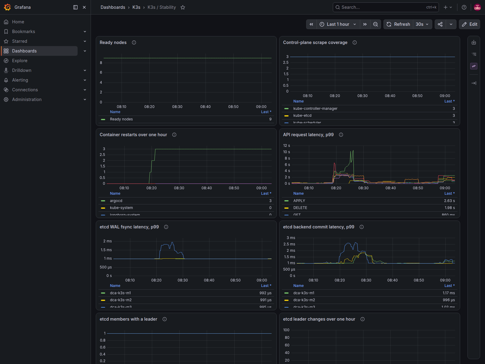
This view shows a one-hour window. All nine nodes remain Ready and each control-plane component has three scrape targets, but the restart and API-latency panels still contain activity worth investigating. Readiness tells me the nodes are available; it doesn’t mean every request was fast or every container ran without interruption. The p99 latency estimates the value below which 99% of the measured requests fall.
Keeping the folders through the next deployment
I kept dashboard JSON under blog-sandbox-argo-cd/observability/dashboards/. The observability/kustomization.yaml file packages each dashboard into a ConfigMap with a grafana_folder annotation identifying the destination folder. The SNMP generator adds the same annotation for Network. Grafana’s sidecar, a helper container, copies those files into the corresponding directories.
Grafana’s file provider checks for dashboard updates every 30 seconds. The sidecar loads the files during startup and continues watching for changes. These settings live in values/victoria-metrics-values.yaml; a Git-managed migration hook removes the old chart-owned dashboards to avoid duplicate IDs.
After deployment, I checked the folders in Grafana and ran all 26 queries on the three new overview dashboards. Each returned data, and browser checks found no query errors or empty panels. The verification record and screenshots show the result.
Reaching Grafana by name
I use
https://grafana.sandbox.lab
for Grafana and
https://argocd.sandbox.lab
for Argo CD. Both names share an ingress address. MetalLB assigns that address to a Kubernetes LoadBalancer Service and announces it on the network; Traefik receives the web request and uses its hostname to select the application.
Browser -> DNS lookup -> ingress IP -> Traefik -> Grafana or Argo CD
The lab has two ingress addresses, one on each network:

The root Application deploys MetalLB, its address pools, Traefik and the application routes from the ingress manifests. The bundled K3s Traefik and ServiceLB remain disabled because I manage this Traefik installation through Argo CD and use MetalLB for address assignment. Two Traefik replicas run on workers in different sites. MetalLB announces the management address on eth0 and the lab address on bond0.
BIND supplies the DNS answers. Its views return the lab address for queries sourced from the lab’s 10.0.0.0/8 network and the management address for management clients. A view is a set of DNS answers selected by the query’s source address. If a resolver forwards the query, BIND sees that resolver’s address.
The names and addresses are declared in blog-sandbox/service_endpoints.yml. To publish them, run the BIND playbook with the existing Nautobot credential environment:
cd /home/ubuntu/blog-sandbox/ansible
.ansible/bin/ansible-playbook pb.dns.yml -e bind_validate_only=true
.ansible/bin/ansible-playbook pb.dns.yml
The first command validates staged DNS configuration without activating it. The second publishes it. My workstation uses pfSense for DNS, so I added a domain override under Services > DNS Resolver > Domain Overrides: sandbox.lab points to the BIND server at 192.168.3.71, with TLS Queries disabled. That destination is the DNS server, not the ingress address. The resolver must also be able to send queries through the management interface.
HTTPS uses a private lab certificate authority (CA), which signs the ingress certificate. After Argo creates the Traefik namespace, the certificate helper creates or reuses the local keys and installs the required Kubernetes Secrets:
cd /home/ubuntu/blog-sandbox-argo-cd
python3 tools/ingress_tls.py
Import the public ingress/lab-ingress-ca.crt into the workstation’s trusted certificate authorities. Private keys stay out of Git. Certificate renewal is a separate maintenance step covered in the ingress runbook.
From the workstation, check the DNS answer and then open Grafana:
nslookup grafana.sandbox.lab
The expected answer is 192.168.3.240. In Grafana, open the Network folder and select Network SNMP. Both Grafana and Argo CD still require their application logins. My ingress checks reached both applications through the lab address from all three datacenters and verified their HTTPS certificates.
Adding routing state to the same collection path
An interface can remain Up while the routing relationship using it fails. That mattered after the troubleshooting companion exposed brief BFD-triggered BGP resets under load. BFD, Bidirectional Forwarding Detection, checks whether a peer remains reachable. BGP, Border Gateway Protocol, exchanges routes and can use BFD to react quickly when a neighbor stops responding. Interface counters alone couldn’t tell me whether those sessions stayed established.
I started by asking the devices what they could return. BGP peer-state queries worked on Cisco and Arista. My first IS-IS query came back empty, but that wasn’t enough to conclude the router couldn’t expose it. IS-IS builds neighbor relationships called adjacencies, and Cisco placed the usable adjacency table under its own MIB branch. A Management Information Base, or MIB, defines the objects available through SNMP; each object has a numeric identifier in that tree. The standard branch and Cisco’s branch were different places to look.
The working Cisco state column was 1.3.6.1.4.1.9.10.118.1.6.1.1.2. I added it to telemetry/routing_metrics.py, alongside BGP state, time established and a counter of entries into Established. Nautobot’s device roles determine which receivers get each profile. The P routers don’t run BGP, so polling an empty BGP table on those four devices would add no useful measurement.
I checked CE1, DCA-Leaf01 and SP1 before expanding. Their existing SNMP access already allowed these reads through the management network. The change was in the collector configuration, deployed through Argo CD, and the samples followed the same path into both VictoriaMetrics stores.
Checking what the numbers actually represented
SP1 exposed five IS-IS adjacencies. To name their interfaces, I followed the circuit index to its IF-MIB index, then used the same full interface description as the interface dashboard. That produced GigabitEthernet2 rather than an unexplained circuit number. The mapping comes from each poll, so I didn’t need to maintain a separate list of circuit-to-port assignments.
BFD caught a problem with that approach. SP1 returned ten SNMP rows, while show bfd neighbors showed five sessions. Each session appeared under two application IDs, 9 and 15. The reported BFD interface indices also disagreed with IF-MIB. Joining those values would have put the wrong interface names beside otherwise plausible Up states.
I kept the BFD local discriminator instead. This is the identifier shown in the CLI’s LD/RD column: LD is the local discriminator and RD is the remote one. The dashboard retains the application rows and counts distinct local discriminators separately. Across the core, 56 application rows represented 28 CLI sessions. I didn’t turn those duplicate rows into extra links or invent protocol names for the application IDs.
The completed polling check looked like this in both metrics stores:
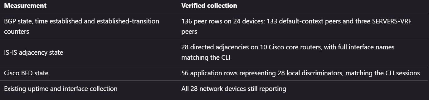
The default SNMP table omitted the SERVERS-VRF peer on each Leaf03 switch. On these EOS devices, polling with the existing community followed by @SERVERS returned the missing peer. I added a BGP-only receiver for each verified context, using the same credential Secret, and checked its state, remote AS, uptime and transition counter against direct SNMP reads. The peer address and Established state also matched show ip bgp summary vrf all.
The collection targets live in telemetry/bgp_vrf_profiles.yaml. The generator verifies that each configured VRF exists on that device’s modeled interfaces in Nautobot. Each measurement carries a vrf label so identical peer addresses in different routing tables remain separate. These metrics cover the verified peer transports; they don’t report how many prefixes each address family exchanges.
Reading the result in Grafana
I added Network Routing beside Network SNMP in the Network folder. BGP rows show the device, VRF, peer address, exact remote AS number and readable state. The BGP VRF selector switches between All, default and SERVERS without changing the IS-IS or BFD panels. Uptime and transition graphs include the VRF in their legends. IS-IS rows show the full local interface name. BFD rows use the local discriminator described above. The dashboard JSON keeps those choices in Git.
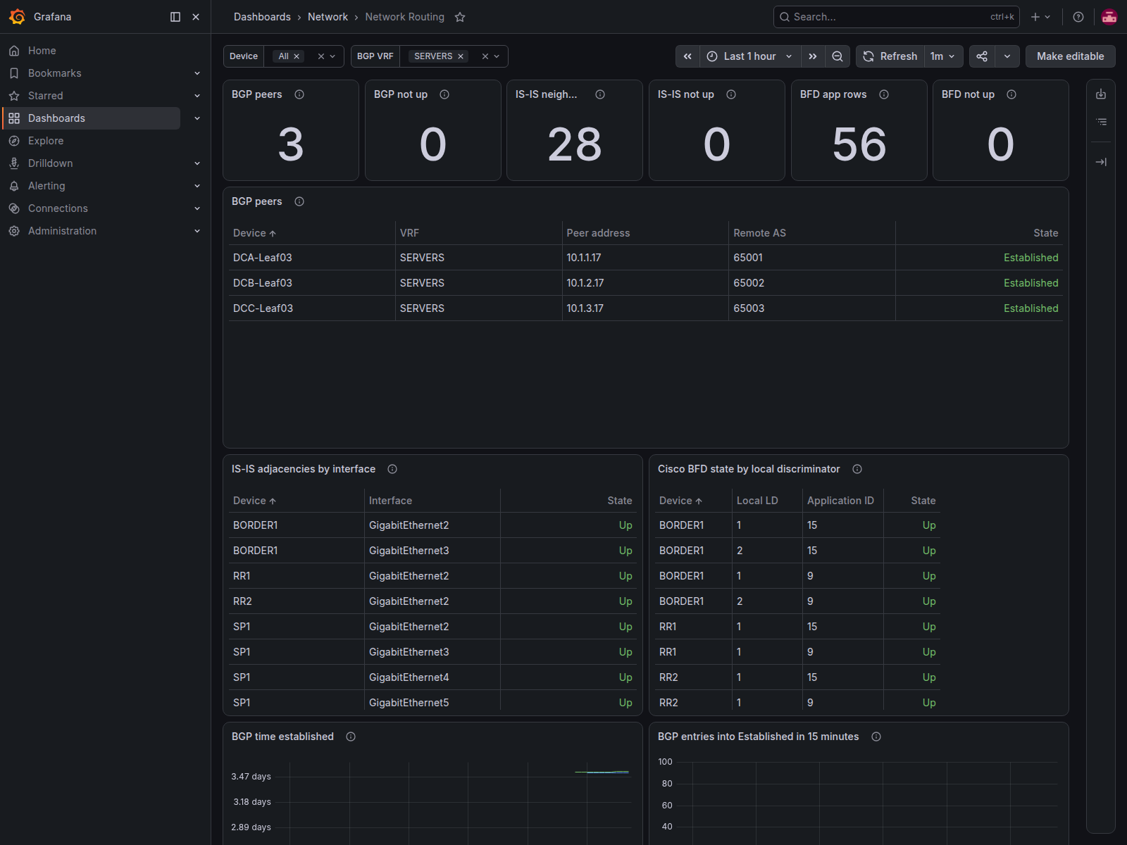
The screenshot selects SERVERS, so it shows three BGP peers. Selecting All shows 136. IS-IS and BFD retain their own counts because the VRF selector applies only to BGP. Remote AS values remain exact numbers, such as 65001, rather than abbreviated measurements.
For the transition graph, I use VictoriaMetrics’ increase_prometheus function to calculate changes between observed counter samples. Starting a new VRF time series must not turn its existing lifetime counter into an apparent burst of recent flaps. The newly labeled graphs begin with this collection rollout; they don’t reconstruct earlier VRF history.
The routing rules also check reported non-up states and row counts below the verified baseline for each device. That second check matters when a failed neighbor disappears from a table instead of remaining there with a Down value. Default-context coverage stays separate from the three SERVERS peers, which also have alerts for a missing device/VRF/peer combination. The baseline must change when I deliberately change the topology. I verified rule evaluation, not delivery to an external notification destination.
What a successful poll still could not tell me
A session can go down and recover between one-minute polls. BGP’s established-transition counter gives me another clue when that happens, but it doesn’t explain why BFD expired. I still need event history beside these graphs.
A poll starts with a request from the collector. An SNMP trap is a notification sent by the device when something happens. Syslog carries event messages, often including the peer, routing context and reason. These need receivers of their own; adding a trap destination to a switch wouldn’t make the OTel SNMP polling receiver accept it.
I checked the notification catalog on the Arista canaries with:
show snmp notification
EOS 4.34.6M listed BGP transitions, interface link-up/link-down and IS-IS adjacency notifications. It didn’t list a BFD notification. Its logs did contain %BFD-5-STATE_CHANGE messages with the peer, VRF and diagnostic reason, so syslog was the source I could follow for those BFD events.
The trap receiving side was still missing. None of the four inspected canaries had an snmp-server host destination, and the cluster had no trap listener or UDP 162 Service. I hadn’t demonstrated end-to-end trap delivery or deliberately interrupted a routing session during these checks.
That next collection path needs a destination reachable through the management VRF, a listener that decodes traps, and syslog ingestion for the BFD details already present on the switches. VictoriaLogs and its planned 14-day retention belong there. I’d start with a safe test notification from one device per platform and check that the stored event retains its device, peer, VRF, interface and reason before expanding.
Knowing whether collection is still working
A Ready collector means its process passed a health check. I also need to know whether a device answered recently. In Grafana’s Explore view, using the SNMP datasource, this query counts devices with an uptime sample less than three minutes old:
count(time() - timestamp(snmp_device_uptime_ticks{job="snmp"}) < 180)
For this fleet, I expect 28. A smaller count tells me to find the stale devices before interpreting their traffic graphs. For interface coverage, I use the same exclusions as the normal dashboard view:
count by (device) (
  snmp_interface_oper_status{
    job="snmp", if_type!="", if_type!="166",
    interface!~"(VoIP-)?Null0"
  }
)
The if_type value 166 identifies the MPLS protocol-layer rows. To inspect a particular port, I select its full name. This query converts the incoming byte counter on CE1’s GigabitEthernet2 into bits per second over a five-minute window:
rate(snmp_interface_in_octets_total{
  job="snmp", device="CE1", interface="GigabitEthernet2",
  if_type!="", if_type!="166"
}[5m]) * 8
The dashboard also shows sample age, polling errors and export queues. A missing sample must remain unknown, not turn into zero traffic. Reported interface speed needs the same care: the speed advertised by a virtual NIC is not a measurement of the virtual topology’s forwarding capacity.
The current verification and screenshots show all ten Argo Applications Synced and Healthy, all nine K3s nodes Ready, and all three Longhorn volumes attached and healthy with three read/write replicas each. Each control-plane component has three successful scrape targets, Longhorn has six and the selected Argo CD components have five. SNMP supplies fresh measurements from all 28 network devices, including 133 default-context and three SERVERS-VRF BGP peers.
I checked the dashboard queries and the pages they render. The three cluster, storage and Argo overview dashboards returned data for all 26 queries; the routing dashboard passed all 45 checks across its All, default and SERVERS selections. Coverage alerts check missing collection, unhealthy volumes and restarts of Longhorn’s storage-driver containers. Rule evaluation works, but delivery to an external notification destination remains untested.
I kept the first release small enough to follow all the way through: one device per platform, a stored measurement, a recognizable interface on a graph, then the rest of the fleet. The startup readback and missing-counter checks showed where a green status could conceal unfinished work. The browser check exposed a different problem: data could be present and still be awkward to use.
I can now select the same interface in Grafana that I would inspect at the CLI and watch its counters while the applications use the network. BGP and IS-IS state now sit beside those counters. Capturing routing events is the next collection step. Flow collection and SuzieQ remain outside this release. The free troubleshooting companion explains the failures that made those measurements necessary; this build gives me the first part of the record for the next investigation.